Robotics Subsystem

The robotics subsystem is a 4-DOF yaw-pitch-pitch-pitch manipulator mounted on the system’s tracked chassis. Its primary purpose is to autonomously recover the biohazard containers and place them upright within the designated Safe Zone. Autonomous operation was chosen to reduce mission time (SYS12) and ensure repeatable accuracy beyond what is achievable through manual teleoperation.

To constrain kinematic complexity, the arm architecture represents the minimum degrees of freedom to satisfy the task. A base yaw joint enables access to biohazards around the chassis, eliminating the need for precise vehicle yaw control. A shoulder-elbow pitch pair supports payload manipulation across a range of elevations. The final wrist pitch joint ensures the payload remains upright at all times.

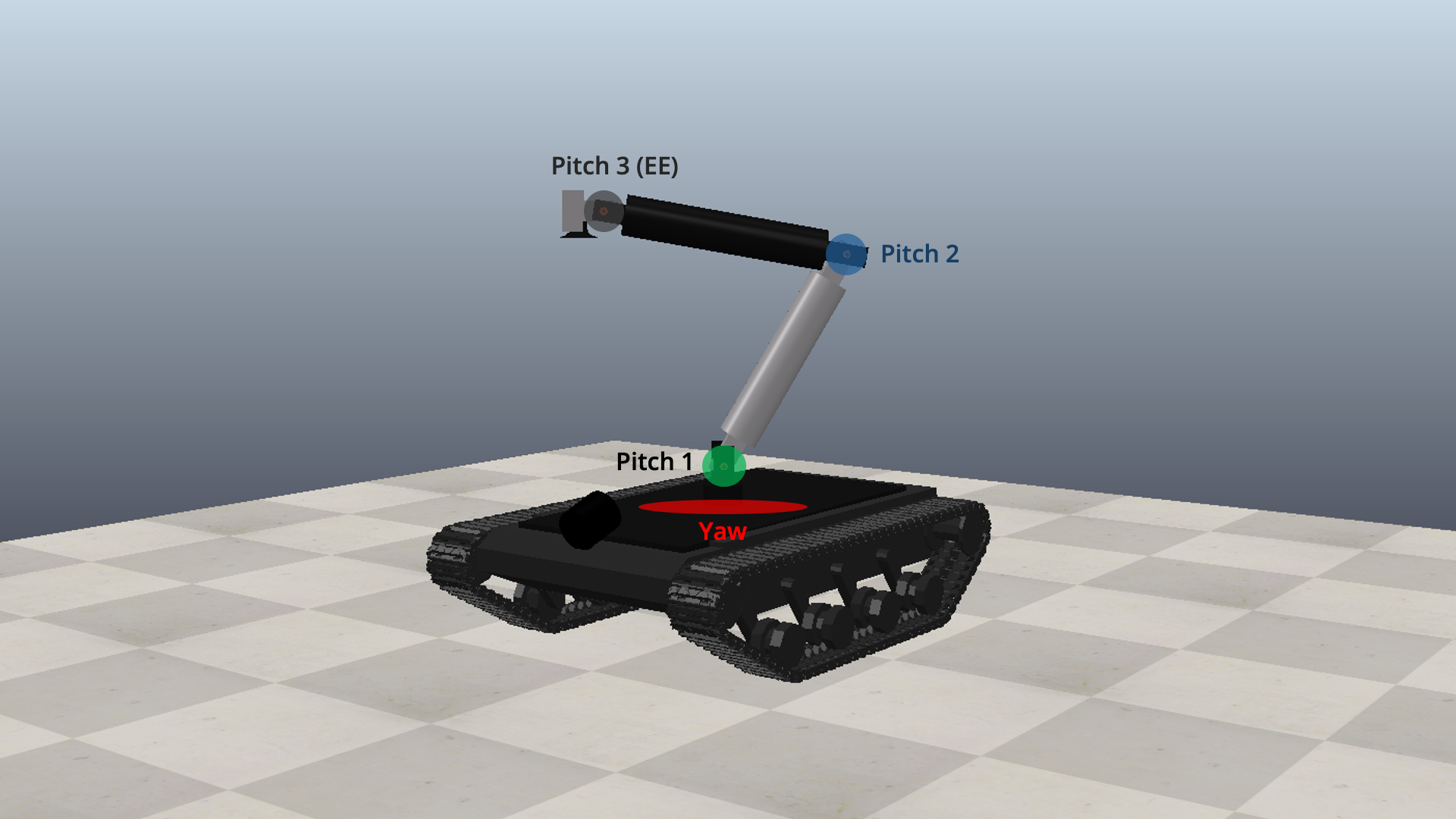
Figure A1 – 4-DOF manipulator design in CoppeliaSim.

A vacuum end-effector was selected after fingered grasping concepts evaluated in CoppeliaSim (Figure A3) proved highly sensitive to contact modelling and unreliable when engaging the 12.75kg payload. A downwards-facing vacuum end-effector instead exploits the payload’s flat lid surface, remaining practically feasible given the availability of industrial vacuum lifters rated well beyond the biohazard mass [1].

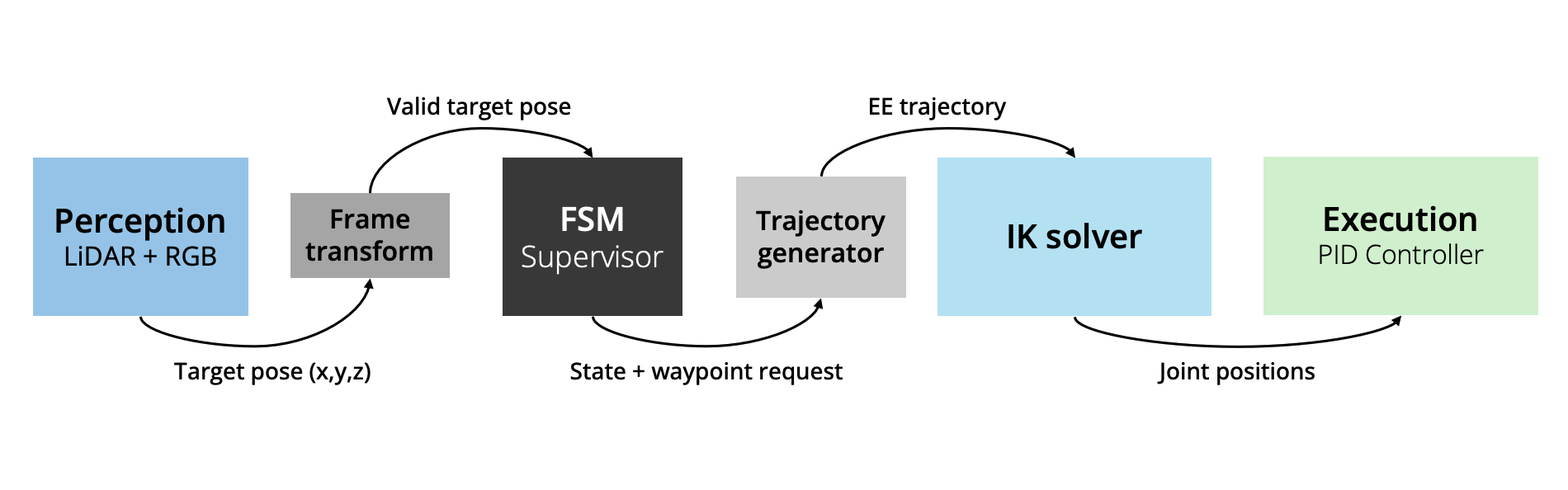
Figure A2 – Robotics system dataflow.

The arm uses an analytical forward and inverse kinematic formulation with PID control, enabling deterministic motion with end-effector tracking error consistently below 0.05 m. Performance is demonstrated through repeated randomised pick–carry–place trials, with placements remaining upright in all cases and a mean cycle time of 18.06s, confirming consistent and time-efficient operation.

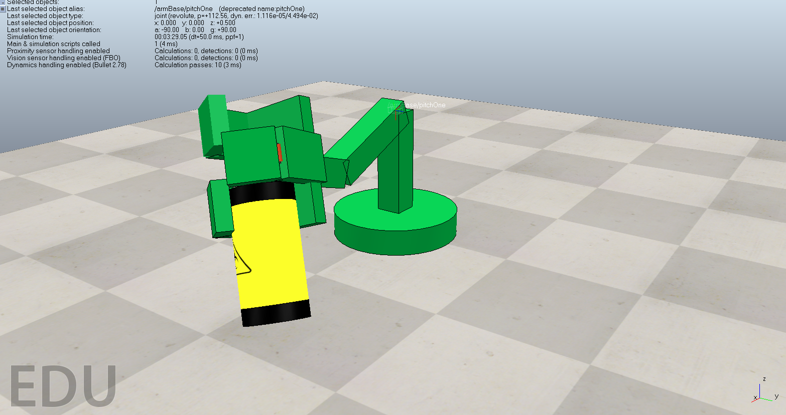
Figure A3 – Trialled gripper end-effector concept.

The robotics subsystem requirements are derived from system level biohazard handling and mission performance objectives, with the aim of enabling accurate and repeatable pick-and-place operation.

Figure B1 – Robotic subsystem requirements.

Although CoppeliaSim employs idealised actuation and simplified contact models, the subsystem will be modelled with high levels of practical fidelity. Structural representation will define explicit geometry, mass and inertia properties, and bounded joint motion consistent with the intended mechanical design.

Arm motion will be governed by analytical kinematic formulations and joint PID control with finite torque and speed limits, ensuring a realistic dynamic response.

Verification is performed by Python driven tests implementing FK/IK, motion sequencing, and joint control, executed using a CoppeliaSim model via the remote API.

Figure C1 – Robotics subsystem test matrix.

D1 Kinematic Architecture

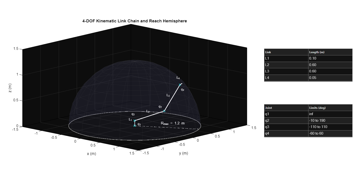
Figure D1.1 – 4DOF kinematic chain and reach hemisphere, including link lengths and joint angle limits.

The robotic arm is implemented as a 4-DOF yaw–pitch–pitch–pitch serial chain mounted on the rover chassis. This configuration was selected to satisfy the biohazard handling requirements whilst minimising kinematic and control complexity.

The base yaw joint (q₁) provides azimuthal coverage. The remaining joints (q₂ - q₄) form a vertical-plane chain that controls reach, height, and end-effector orientation. Decoupling the base yaw from an equivalent planar 3R chain enables a fully analytical inverse kinematic solution without reliance on numerical solvers.

This avoids common numerical failure modes such as sensitivity to initial guesses, convergence issues and singularity hunting, providing a fast and robust system for autonomous pick and place.

Geometric and joint constraints

Link lengths were selected to satisfy the reach requirement (R01) whilst keeping the arm compact when folded. The final arrangement comprises a short base offset, two primary reach links, and end-effector (Figure D3).

Joint limits were defined to remain physically realistic and to prevent non-representative postures in simulation. These were implemented within CoppeliaSim joint properties so that subsequent IK and control results are generated under the correct, constrained motions. (Figure D1.2)

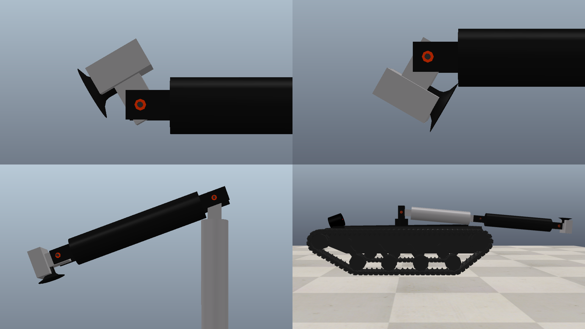
Figure D1.2 – Joint limits were defined and set in CoppeliaSim, to eliminate unrepresentative motion. Numerical values in Figure D1.1.

Task pose feasibility

The reachable range is \(R_{\max}=1.2\,\mathrm{m}\) around the base (Fig. D1). The hemisphere envelope was used to confirm, at architecture stage, that the arm can achieve the three poses required without operating at extreme joint limits:

• Pickup Pose:end-effector positioned above a ground-level container with a top-down approach.
• Carry Pose:payload raised within the rover for motion over uneven terrain.
• Placement pose:end-effector positioned within the safe zone with a controlled approach suitable for vertical deposition.

 

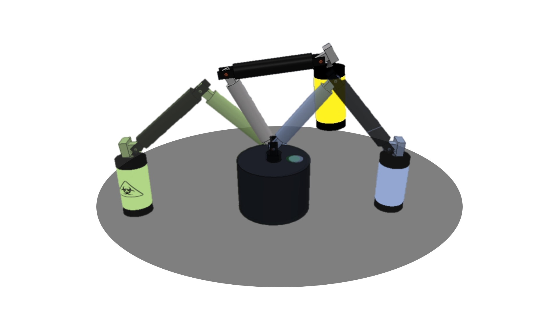
Figure D1.3 – Pickup, carry and placement pose.

 

D2 Kinematics and Motion Control

This section presents the kinematic models and joint control strategy used to operate the autonomous robotic arm architecture defined in Section D1.

1. Kinematic calculations, trajectory generation and task sequencing are implemented in Python and executed externally to CoppeliaSim via the ZMQ Remote API.
2. CoppeliaSim provides the rigid-body dynamics, joint limits and joint state feedback.

Python excerpts are included to evidence the implementation; full scripts are attached in the comments.

D2.1 Forward kinematics

Forward kinematics map a given joint configuration to the end-effector position and orientation in the world frame: \[ q = [q_1,\; q_2,\; q_3,\; q_4]^T \]

The model uses standard homogeneous transforms for the base yaw and the planar 3R chain. The overall transform from base frame \(\{0\}\) to end-effector frame \(\{E\}\) is written in compact form as \[ {}^{0}T_{E}(q)=T_{\mathrm{yaw}}(q_{1})\,T_{2}(q_{2})\,T_{3}(q_{3})\,T_{4}(q_{4}) \]

from which the Cartesian position \((x,\;y,\;z)\) and planar end-effector angle \(\phi_{\mathrm{pad}}\) are extracted. In implementation, forward kinematics lies within the software framework at robotics/FK.py.

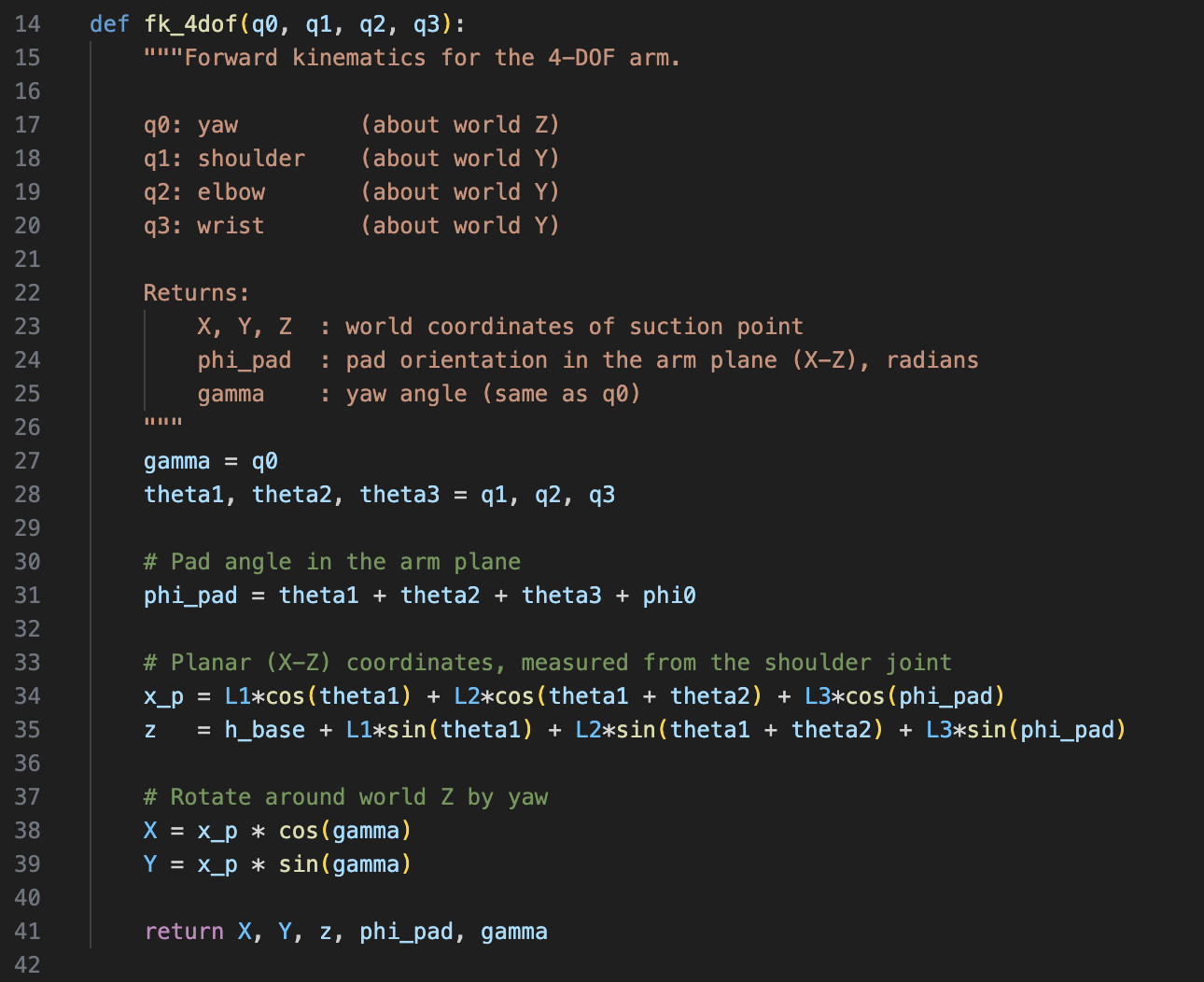
Figure D2.1 – Excerpt of Python implementation of forward kinematics.

D2.2 Inverse kinematics with vacuum pad down constraint

Inverse kinematics (IK) compute a joint configuration \(q\) that realises a desired end-effector pose: \[ (x_{\mathrm{des}},\,y_{\mathrm{des}},\,z_{\mathrm{des}},\,\phi_{\mathrm{EE,des}}) \]
To meet the vertical biohazard placement requirement, the vacuum pad at the wrist is constrained to point approximately downwards, so the end-effector angle is fixed to \[ \phi_{\mathrm{EE,des}}=-\frac{\pi}{2} \]

With this constraint, the 4-DOF IK separates into three steps:

1) Base yaw
The base joint aligns the arm with the target in the horizontal plane: \[ q_{1}=\operatorname{atan2}\!\left(y_{\mathrm{des}},\,x_{\mathrm{des}}\right) \]

2) Planar 2-link solve; shoulder and elbow
The target is projected into the arm plane using the radial distance and height: \[ r=\sqrt{x_{\mathrm{des}}^{2}+y_{\mathrm{des}}^{2}},\qquad z' = z_{\mathrm{des}}-h_{\mathrm{base}} \]

Because the end-effector orientation is fixed, the wrist joint is offset from this point along the vertical direction, giving an equivalent wrist-centre \((x_w, z_w)\). A standard 2-link elbow solution (law of cosines) is then applied to find \(q_{2}\) and \(q_{3}\) for link lengths  and .

3) End effector (wrist) angle
The wrist closes the kinematic chain so that the end-effector remains vertical:

\[ q_{2}+q_{3}+q_{4}=\phi_{\mathrm{EE,des}} \]

\[ q_{4}=\phi_{\mathrm{EE,des}}-q_{2}-q_{3} \]

The solver returns both the joint vector and a “reachable” flag. Targets outside the 1.2m workspace or violating joint limits are rejected, preventing the controller from trying to achieve unfeasible poses and freezing mid-manoeuvre.

In code, the inverse kinematics are implemented using a closed-from solver. This ensures fully deterministic motion planning, and therefore the immediate identification of infeasible targets as law-of-cosines violations.

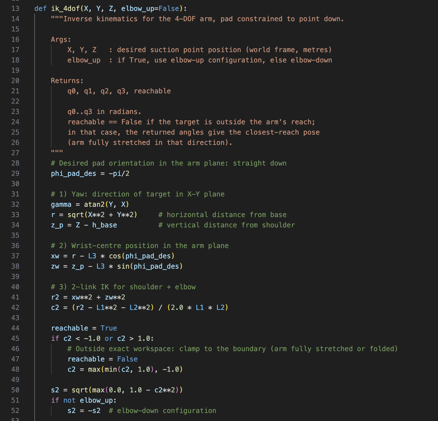
Figure D2.2 – Excerpt of inverse kinematics Python function.

D2.3 Task trajectory and autonomous manipulation of biohazard

Pick-carry-place motion is generated as a sequence of time parameterised waypoints evaluated through the IK solver. Figure D2.3 shows the state machine.

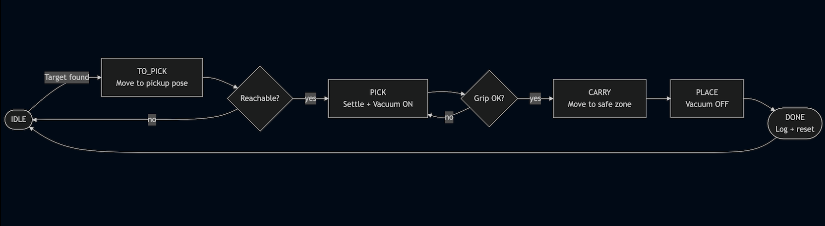
Figure D2.3 – Simplified pick-carry-place finite-state machine (FSM).

Half-cosine interpolation provides smooth joint commands with zero boundary velocity. In CoppeliaSim, motion is constrained by the applied joint torque and velocity limits, defined by the motor selections in the Mechatronics subsystem. This ensures realistic behaviour as much as possible.

Figure D2.4 – Video of autonomous pick-up, hold and placing of biohazard.

D2.4 PID control and tuning

Each joint tracks its commanded position using an internal PID controller within CoppeliaSim.

At runtime, Python computes desired joint angles \(q_{\mathrm{ref}}(t)\) from the analytical IK solver and commands them via sim.setJointTargetPosition(). The simulator closes the control loop using measured joint position \(q(t)\), yielding a standard control law:

\[\,e_{\theta}(t)=q_{\mathrm{ref}}(t)-q(t)\]

Each joint is regulated by its own \((K_p,\,K_i,\,K_d)\). This allows individual joint controller performance to be evaluated objectively before validating full pick–carry–place manoeuvres.

Figure D2.5 – Automated joint controller tuning via Python.

The internal PID controllers were tuned via an automated Python routine, by executing repeatable step-response tests and logging joint motion (Figure D2.5). Each tuning run applies a step from \(0^\circ\) to a configurable target angle \(\theta_{\mathrm{step}}\). For each candidate gain set, the script records:

• joint angle \(\theta(t)\) for tracking performance.
• joint torque\(\tau(t)\) to verify compliance with joint

Python-controlled stepping is used to ensure consistent sampling and repeatability across runs.

Objective function

Each response is reduced to a scalar cost: \[ J=\mathrm{RMS}(e_{\theta})+\max(0,\mathrm{OS})+2\,e_{\mathrm{ss}} \]

• \(\mathrm{RMS}(e_{\theta})\) is the RMS tracking error
• \(\mathrm{OS}\) is overshoot
• \(e_{\mathrm{ss}}\) is steady-state error

This formulation penalises poor tracking, oscillation, and residual bias.

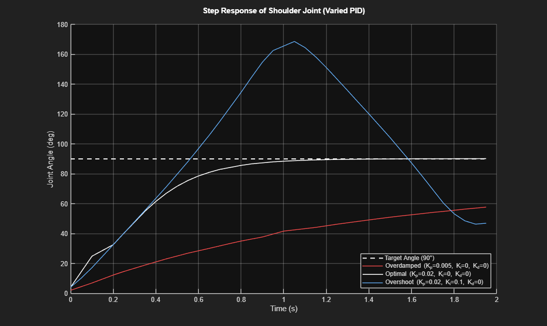
Figure D2.6 – Step response of shoulder joint with varying PID parameters.

Tuning strategy

To maintain robustness and transparency, gains are selected using a structured sweep that mirrors manual tuning:

1. sweep \(\,K_p\,\) with \(\,K_i=K_d=0\,\)
2. sweep \(\,K_d\,\) with \(\,K_p\,\) fixed at its optimal value
3. sweep \(\,K_i\,\) with \(\,K_p, K_d\,\) fixed

Selected gains for each joint

Figure D2.6 shows representative shoulder joint step responses before and after tuning. The selected gains achieved a settling time of 1.2s, with negligible overshoot and low steady-state error (\(e_{\mathrm{ss}}=0.075^\circ\)). This exceeds requirement R06 (\(T_s \le 2\,\mathrm{s}\)s, \(\mathrm{OS} \le 20\%\), \(e_{\mathrm{ss}} \le 2^\circ\)) with clear margin.

The final gain set used in simulation is summarised in Table D2.4; full CSV data is provided in the comments.

Figure D2.7 – Finalised PID values for individual CoppeliaSim joint controllers.

 

D3 Structural and materials design

The arm links are dimensioned using a von Mises structural analysis, with link masses and inertias derived from feasible physical sections. This ensures that the CoppeliaSim model produces joint torques and motion behaviour representative of real hardware.

All links are modelled as hollow 6061-T6 aluminium tubes:

• The material is widely available and established in robotic applications [2], providing a high stiffness-to-weight ratio together with favourable manufacturing characteristics.
• Mild steel was considered as an alternative; however, it offers no functional advantage for this application. Steel would significantly increase link mass and torque demand, penalising dynamic performance.
• Carbon-fibre tubes could reduce mass further, but at the cost of substantially increased manufacturing and integration complexity. [3][4]

D3.1 Design load case and constraints

Structural sizing is based on a worst-case manoeuvre that maximises combined gravitational and inertial loading:

12. The arm is fully extended horizontally carrying the 12.75kg biohazard
13. The shoulder joint pitches from 0° to 90° over 1s using a cubic motion profile

Only the primary pitch links (L1 and L2) are sized explicitly, as they dominate bending span and loading. The selected tube section is then reused for the remaining links to simplify modelling and remain conservative.

Link lengths are taken from a geometry that accounts for joint housing rather than kinematic lengths, as these increase the effective bending span. Figure D3.1 shows the resulting CoppeliaSim geometry with overlapping links.

For each candidate tube section, a MATLAB sizing script evaluates:

• Joint torque demand
• Maximum von Mises bending stress
• Static and dynamic tip deflection
• Torsional twist

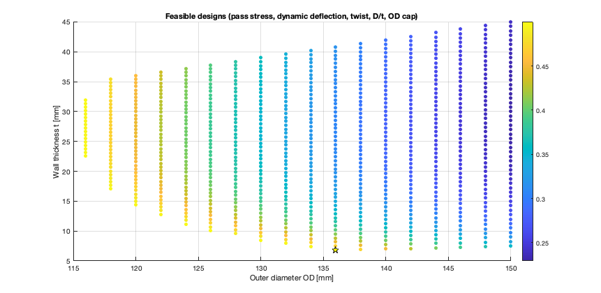
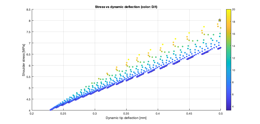
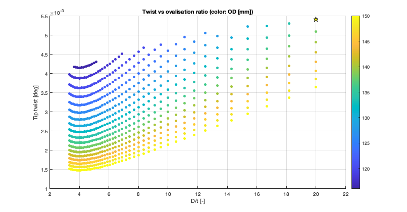
Candidate sections are swept parametrically in outer diameter and wall thickness. Each section is assessed against the structural constraints listed in Figure D3.2. Among feasible designs, the section with the lowest combined mass is selected.

A yield safety factor of 2.0 is applied to cover modelling simplifications, such as motor masses and idealised joints. Full parametric sweep results are provided in Figure 3.4 and Appendix R1.

Figure D3.2 – Structural evaluation criteria.

D3.2 Selections

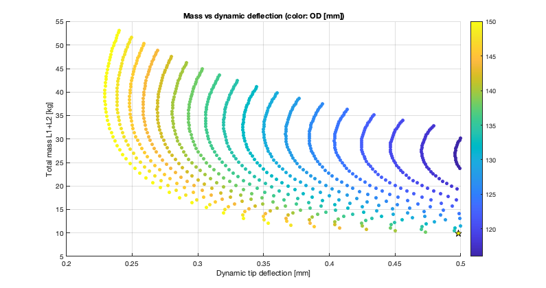
Figure D3.3 – Mass vs stiffness sweep visualisation; colour indicates outer diameter. The selected section indicated by a star is the lightest design which meets the deflection target.

Figure D3.4 – Selected link geometry balanced between mass and strength/stiffness requirements.

The optimised selection (Figure D3.4) is the lightest configuration that met the strength and stiffness constraints.

The resulting mass and inertia values for each link were then modelled in CoppeliaSim to ensure a representative arm. The design torque values determine the motor selections in the Mechatronics Section.

 

Figure E1 – Robotics subsystem test result matrix.

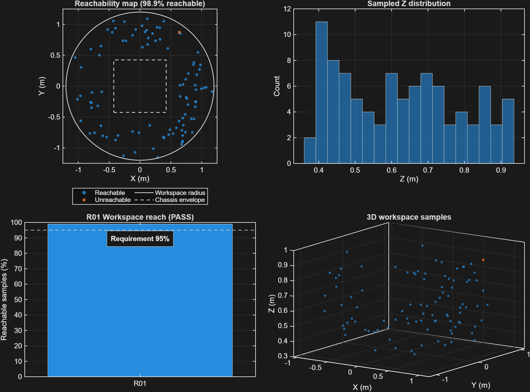
Figure E2 – R01 manipulator workspace reachability of 98.9%.

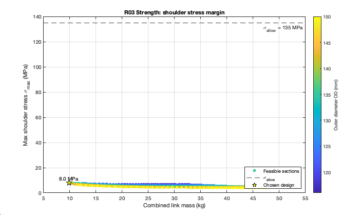
Figure E3 – R03 structural strength margin.

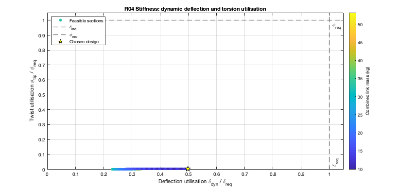
Figure E4 – R04 end-effector stiffness performance.

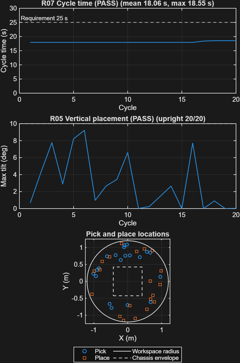
Figure E5 – R05, R07 Vertical placement and cycle data for autonomous trials.

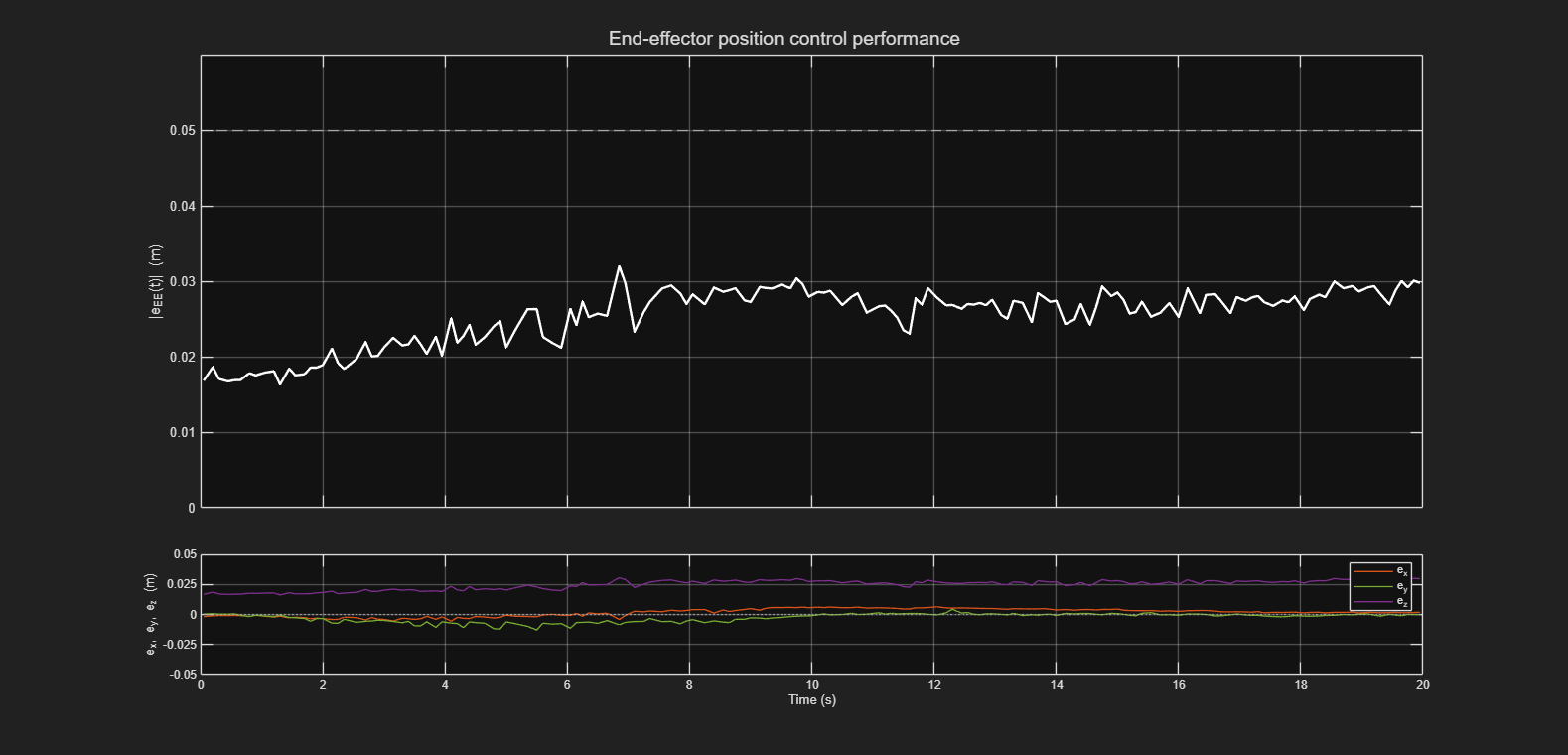
Figure E6 – R06 End-effector x,y,z position accuracy.

 

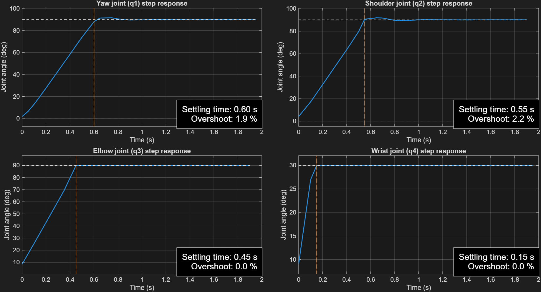
Figure E7 – R06 Individual joint step responses.
Step responses of joints q1–q4 showing settling time and overshoot.

 

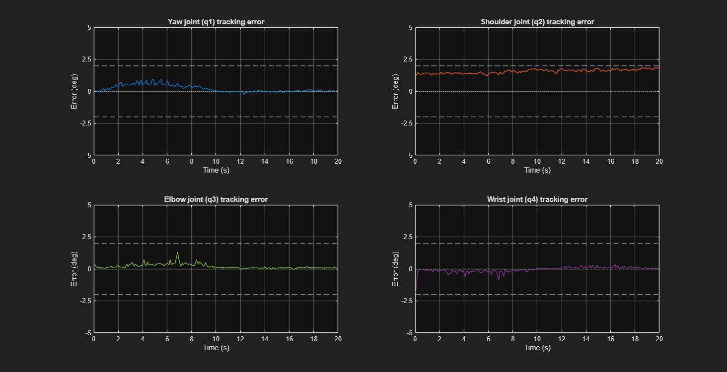
Figure E8 – R06 Joint tracking accuracy.
Joint tracking error for q1–q4 during autonomous operation, with ±2° bounds indicated.

 

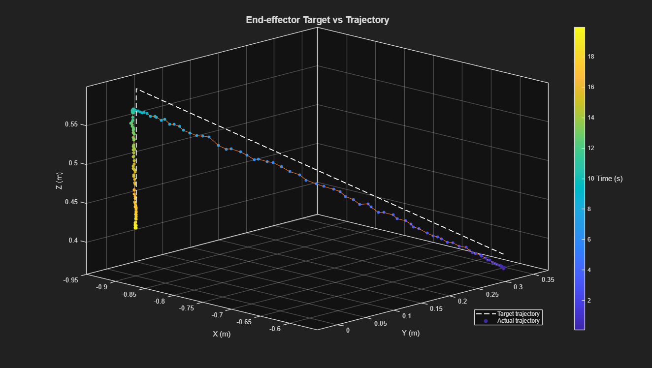
Figure E9 - End-effector trajectory tracking.

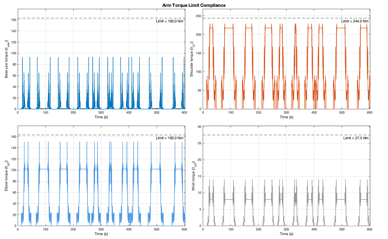
Figure E10 - R08 actuator limit compliance.

Figure E11 – Randomised autonomous pick-place demonstration video (used for R01, R02, R05 and R07).

A scripted manoeuvre test executed randomised autonomous pick-place cycles within the valid workspace, verifying reachability, payload retention and cycle completion time.

The 4-DOF manipulator design satisfies its core objective, repeatedly achieving autonomous recovery and placement of the 12.75kg biohazard. End-effector tracking error remains below 0.05m throughout repeat testing, with a mean pick–place cycle time of 18.06s. At system level, these outcomes de-risk the mission time requirement (SYS12), allowing the operator to focus on navigation and perception.

Real-world deployment considerations informed the design. An analytical IK/FK formulation avoids numerical non-convergence and provides predictable behaviour under timing jitter, while vacuum grasping significantly reduces sensitivity to small pose errors related to fingered grasping. Nonetheless, the simulation assumes ideal surface conditions. In practice, dust or moisture will degrade seal quality. A deployable system would require vacuum pressure sensing to detect loss of seal, or a passive mechanical feature to prevent payload drop in the event of suction failure.

The system exhibits clear structural margin across its requirements. Even under increased loading, first-order scaling indicates stresses remain far below allowable limits. For example, a 20kg payload would result in a peak link stress of 12.5MPa, compared to a 135MPa allowable limit. This demonstrates that the design is tolerant to reasonable requirement changes.

References:

[1] J. Schmalz GmbH, “Vacuum Lifting Device VacuMaster,” Schmalz. Accessed: Jan. 02, 2026. 

[2] J. R. Davis, Aluminum and Aluminum Alloys. Materials Data/NIST (PDF). Accessed: Jan. 02, 2026. 

[3] Aalco, “Aluminium Alloy – Commercial Alloy – 6061 – T6 Extrusions (datasheet),” Accessed: Jan. 02, 2026. 

[4] Composites UK, “Mould Tooling for Fibre Reinforced Polymer Composites,” (Good Practice Guide, PDF). Accessed: Jan. 02, 2026.

 

Appendix:

R1 - Additional structural sweep plots