Sensors Subsystem

The system design uses a tracked rover for biohazard recovery, and a quadcopter drone to support aerial mapping and geolocation. The sensor subsystem’s core responsibilities are to:

1. Provide continuous 360° navigation and obstacle awareness for the ground robot
2. Deliver 3D target geometry for autonomous biohazard manipulation
3. Inform the operator via live spatial visualisation and aerial mapping
4. Measure internal system states such as joint position and chassis orientation

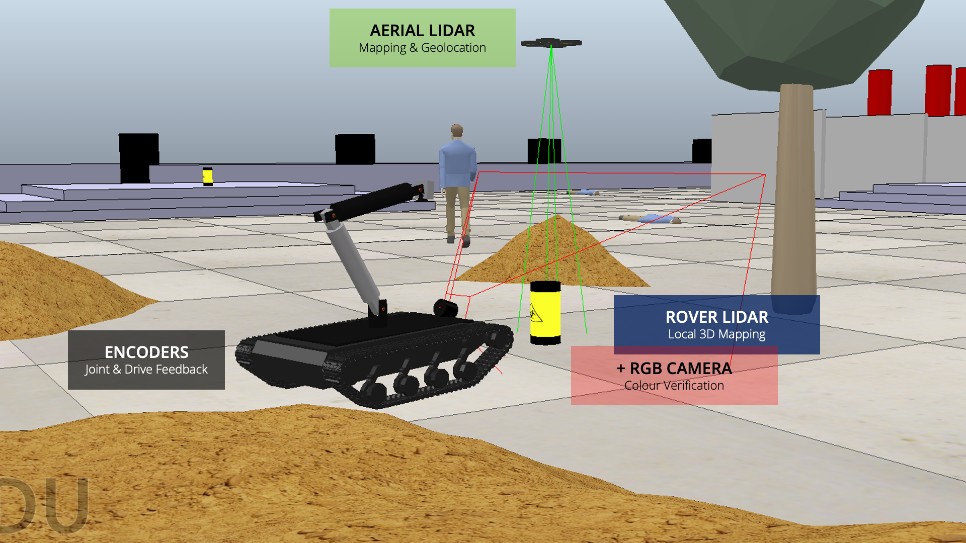
Figure A1 – Sensor suite placement in overall system design.

A 3D LiDAR is selected as the primary perception sensor on the rover and drone. The biohazard environment is characterised by smoke, fire, and degraded visibility, therefore wholly appearance-based alternatives such as RGB vision were deemed unreliable. [1-4]

LiDAR systems produce metrically accurate, lighting invariant XYZ data, enabling robust mapping and localisation via SLAM principles; the simulated LiDAR concept utilises clustering and model fitting to achieve highly accurate object detection (DBSCAN & RANSAC). The approach delivered >95% biohazard detection with worst case positional error below 5mm, while the drone-mounted LiDAR provided aerial mapping with 0.1m geolocation accuracy across the 50×50m arena.

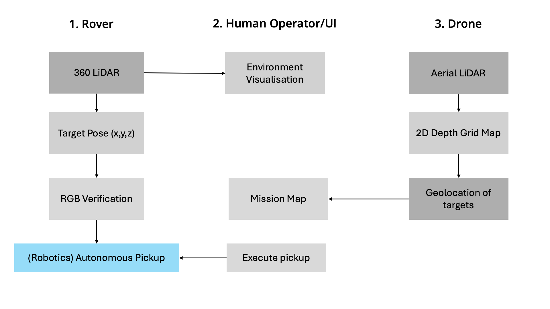
Figure A2 – Sensor data flow and decision logic.

To mitigate false positives at close range, additional RGB sensing was implemented for appearance-based verification prior to autonomous pick-up.

In practise, joint encoders and an end-effector IMU will provide internal state for arm control, but in simulation these are read directly from CoppeliaSim joints, so this topic is instead evaluated in the Robotics Section with regards to control.

The sensor requirements in Figure B1 are derived from system-level objectives, including biohazard recovery, casualty detection and time efficient mission completion. Each subsidiary requirement defines what the simulated sensor suite must achieve to support required functionality, while the final column notes how considerations for real deployment.

Figure B1 Sensor subsystem requirements table.

Figure C1 – Sensor subsystem test matrix.

The sensor subsystem will be tested via automated parameter sweeps and scenario runs in CoppeliaSim. While this enables rapid and repeatable evaluation, the results are optimistic because the simulated sensors are noise free and the environment idealised.

D1 LiDAR geometry and data flow

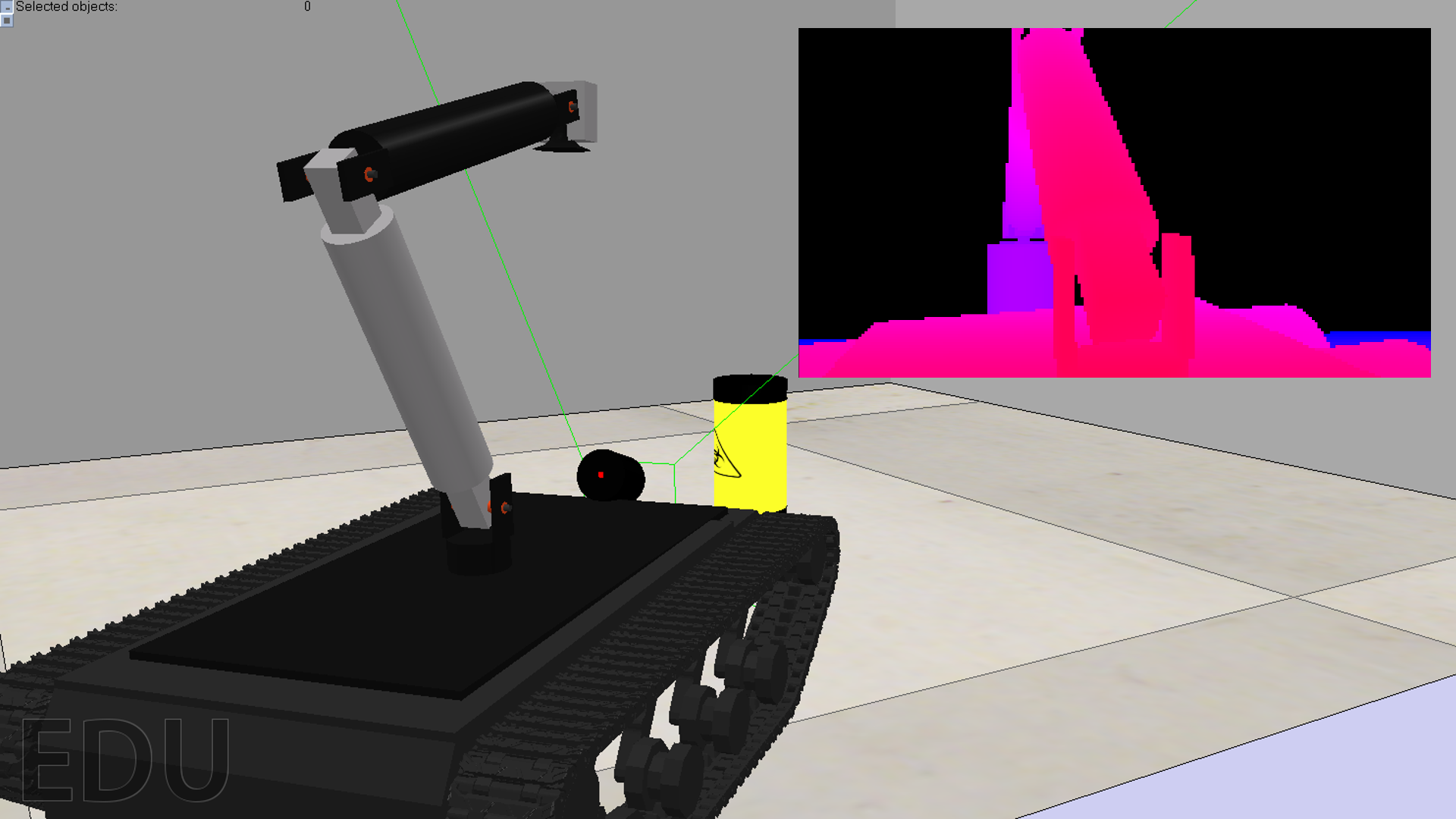
Figure D1.1 – CoppeliaSim rover LiDAR placement and depth visualisation feed.

The tracked ground robot and drone simulate a LiDAR via a CoppeliaSim perspective vision sensor; the data is processed via an external Python framework (in Portfolio comments). Each pixel \((u,v)\) returns a depth value \(d\) along the observed ray. A pinhole model was implemented to transform this into a 3D point within the sensor frame: \[ p_{L}=d\,K^{-1}\begin{bmatrix}u\\v\\1\end{bmatrix} \]

Where \(K\) is the intrinsic matrix from field-of-view and resolution. Points are then transformed into the robot or world frame using a rigid transform as follows: \[ p_{W}=T_{WR}\,T_{RL}\,p_{L} \]

with \(T_{RL}\) the LiDAR robot calibration and \(T_{WR}\) as the robot pose.

Depth images are streamed via the ZMQ Remote API, reshaped with numpy into a point cloud, and then passed through a processing pipeline as follows:

1. Down sampling
2. Ground removal
3. Clustering
4. Model fitting
5. Target list

 

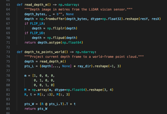
Figure D1.2 – LiDAR depth acquisition and world-frame point-cloud projection (abridged).

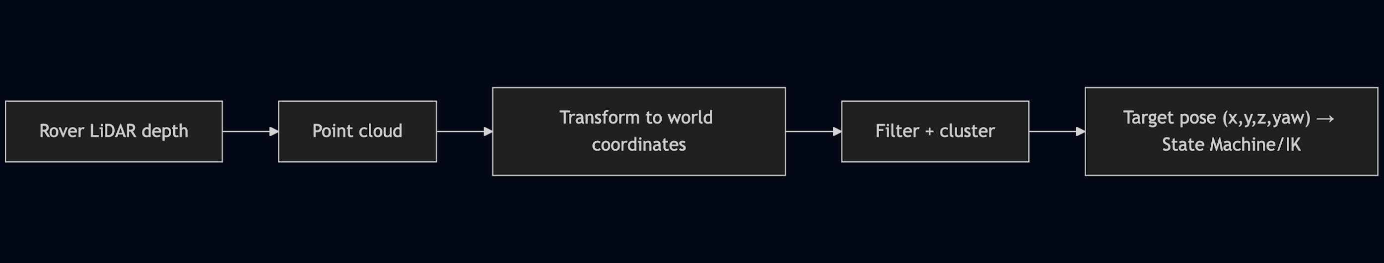
Figure D1.3 – LiDAR signal flow diagram.

 

D2 Biohazard detection and position estimation

Starting from the world-frame point cloud generated in Section D1, biohazard positions are estimated through a structured filtering, clustering and model-fitting pipeline:

1) The raw point cloud is voxel-filtered to reduce noise whilst preserving the cylinder silhouette, with a finer voxel resolution applied close to the robot where position accuracy is most critical.

2) Ground-plane removal and height gating discard points below the expected pick-up region (\(z=0.20\,\mathrm{m}\)), preventing floor points from dominating clusters.

3) The remaining points are clustered using DBSCAN to identify candidate objects. DBSCAN was chosen because it does not require a predefined cluster count and is robust to isolated noise points.

4) For each cluster, a RANSAC cylinder model is fitted. Clusters with low residual are accepted as cylinders, and high-error fits are labelled “uncertain” and ignored.

The average residual is:

\[ e_{\mathrm{cyl}}=\frac{1}{N}\sum_{i}\left|\ \left\|\,(p_i-c)-\big((p_i-c)\cdot\hat{a}\big)\hat{a}\,\right\|-r\ \right| \]

where \(c\) is a point on the axis, \(\hat{a}\) the axis direction and \(r=0.10\,\mathrm{m}\) the nominal radius.

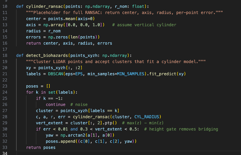
Figure D2.1 – Simplified DBSCAN + RANSAC cylinder detector.

Parameter sweeps using an automated positioning script were used to tune voxel resolution, DBSCAN parameters, and height gating (example CSV in comments). Early configurations exhibited a floor to object “bridging” behaviour, where ground returns merged with the cylinder.

This was mitigated by tightening the height gate and rejecting clusters with implausible vertical extent. Within the resulting sensor range, a >95% detection rate was achieved, with mean absolute position errors below 5cm (Section E Test Results).

For each accepted cylinder, the estimated world-frame pose (x, y, z, yaw) is passed directly to the inverse-kinematics state machine as the pickup target.

Figure D2.2 – Autonomous biohazard pickup using LiDAR derived position.

 

D3 LiDAR depth-map visualisation

To support teleoperation in the low-visibility environment, the rover LiDAR output is visualised as a depth map. Sensor data is streamed to an external Python process for real-time visualisation, where a high-resolution colour gradient conveys relative distance to support obstacle awareness. The display updates synchronously with CoppeliaSim, with non-finite range returns masked.

Figure D3 – Rover LiDAR depth-map teleoperation view.

 

D4 Aerial LiDAR mapping and geolocation

The quadcopter performs an automated aerial survey, using a downward-facing LiDAR to acquire depth images of the full environment. Each depth image is converted to a world-frame point using the projection pipeline defined in Section D1. In simulation, the drone and rover positions are read directly from their object transforms; in practice this would be estimated by a combination of GNSS and SLAM techniques.

Figure D4.1 – Aerial LiDAR depth map and geolocated biohazards/casualties over the arena.

Points are projected onto a fixed  grid and accumulated to form a 2D depth map. DBSCAN and simple geometric checks are then applied to extract clusters corresponding to biohazards and casualties.

Detected biohazards and casualties are stored as global markers and updated live within a shared world frame, alongside the rover position, allowing the operator to assess target locations, quantities, and vehicle motion on a single map. This satisfies SEN04 and contributes directly to system-level geolocation requirement SYS11.

 

D5 RGB Verification:

An RGB camera is mounted on the robot chassis, processed by Python to confirm LiDAR detections (code in comments). Each frame is converted to HSV and thresholder for yellow (biohazard) and green (safe zone). A central ROI is used so only objects directly ahead are considered. If enough pixels are seen near a LiDAR marker, the object is confirmed.

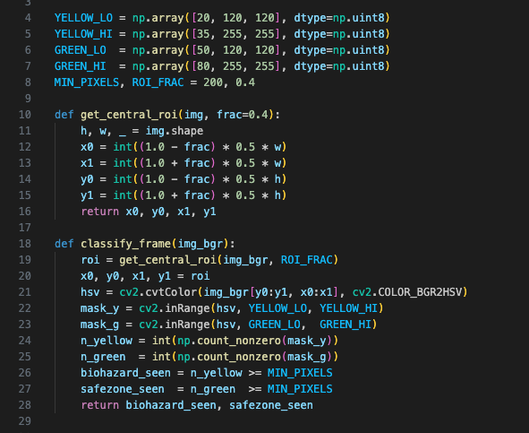
Figure D5.1 – Colour thresholding code.

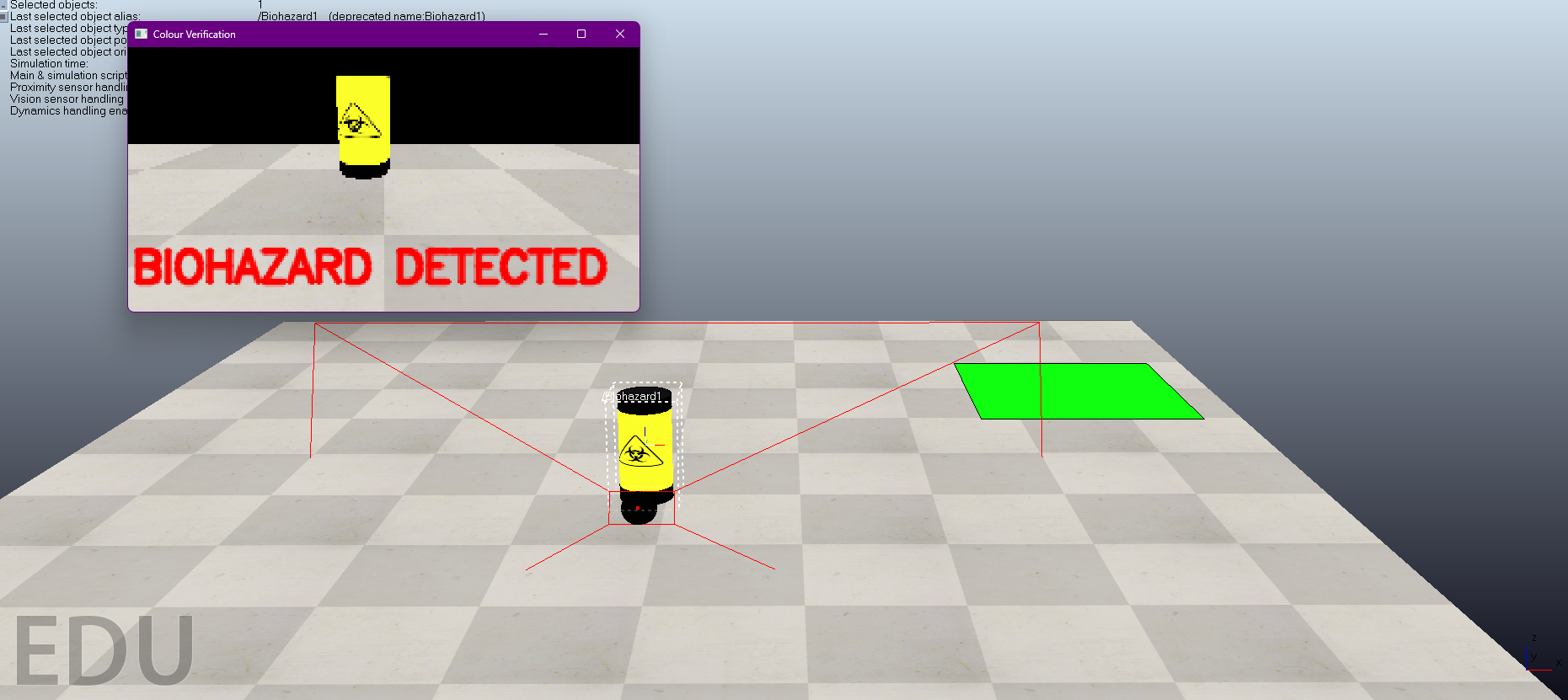
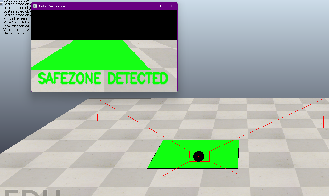
Figure D5.2 – RGB frames and HSV masks.

 

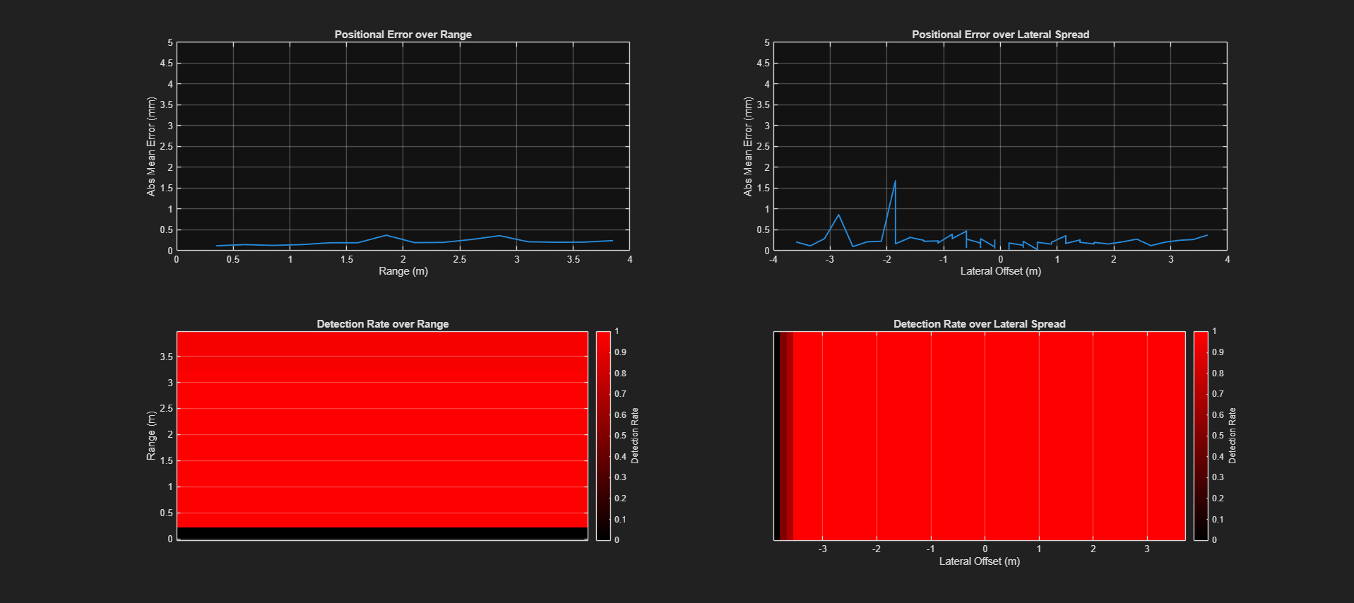
Figure E1 – Rover LiDAR detection & error.

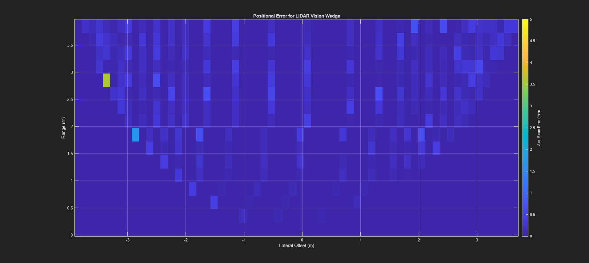
Figure E2 – LiDAR positional error heatmap.

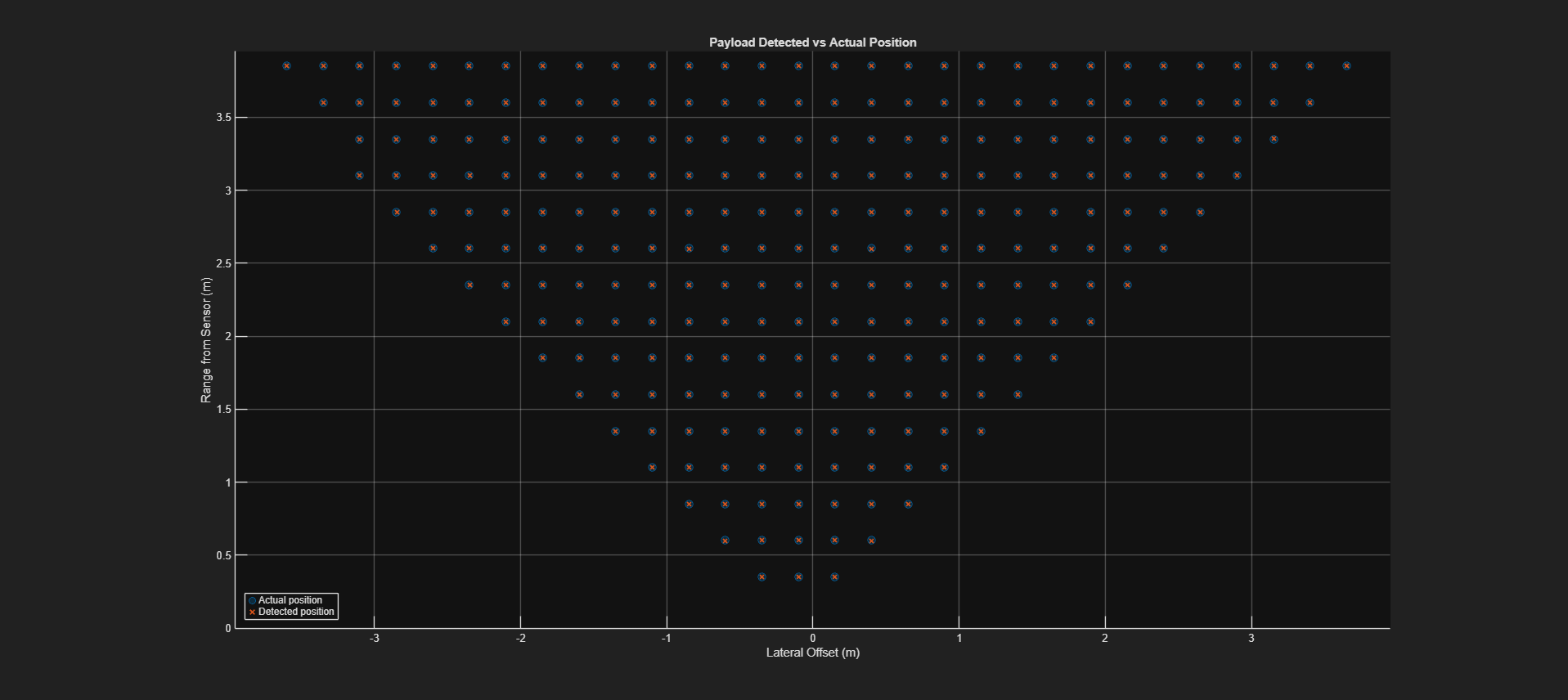
Figure E3 – Detected vs actual payload positions.

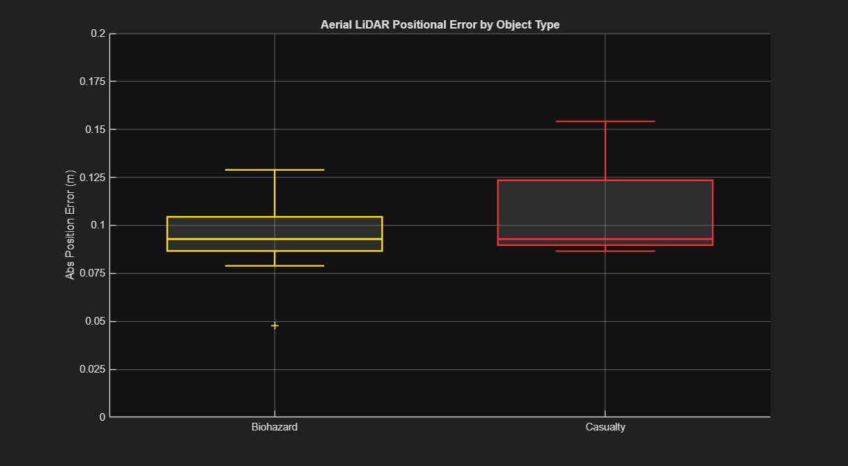
Figure E4 – Aerial LiDAR boxplot positional error by object type.

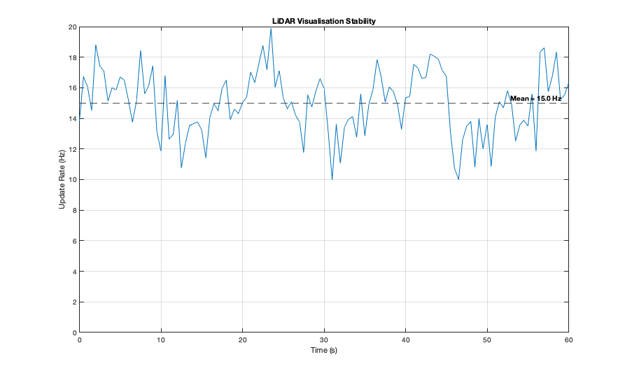
Figure E5 – LiDAR visualisation stability.

The forward-sector LiDAR configuration was a compromise driven by CoppeliaSim performance limits. In practice, this would be replaced by a 360° LiDAR to support omnidirectional environment awareness.

Simulation results are optimistic and will degrade in practice due to noise, misalignment, and environmental interference. These effects can be mitigated through sensor–robot calibration, the retuning of detection thresholds using noisy test data, and the deliberate use of redundant sensing. This redundancy is partially demonstrated within the simulated concept: LiDAR provides primary spatial perception, while RGB vision acts as an independent close-range confirmation step.

Notwithstanding these limitations, the designed sensor subsystem demonstrates a balance between robustness and computational complexity, providing a credible foundation for a real-world biohazard response system.

[1] R. Siegwart, I. R. Nourbakhsh, and D. Scaramuzza, Introduction to Autonomous Mobile Robots, 2nd ed. Cambridge, MA, USA: MIT Press, 2011.

[2] M. Ester, H.-P. Kriegel, J. Sander, and X. Xu, “A density-based algorithm for discovering clusters in large spatial databases with noise,” in Proc. 2nd Int. Conf. Knowledge Discovery and Data Mining (KDD), 1996, pp. 226–231.

[3] M. A. Fischler and R. C. Bolles, “Random sample consensus: A paradigm for model fitting with applications to image analysis and automated cartography,” Commun. ACM, vol. 24, no. 6, pp. 381–395, Jun. 1981, doi: 10.1145/358669.358692.

[4] C. Cadena et al., “Past, Present, and Future of Simultaneous Localization and Mapping: Toward the Robust-Perception Age,” IEEE Trans. Robot., vol. 32, no. 6, pp. 1309–1332, Dec. 2016, doi: 10.1109/TRO.2016.2624754.